A guide to solar energy yield assessment

The transition from a preliminary site concept to a bankable solar asset depends on a single variable: the accuracy of your energy yield assessment. In the gigawatt era, where project margins are razor-thin, treating yield as a "fixed number" is a strategic liability. This guide explores the technical frameworks required to simulate, calculate, and optimize solar energy production for maximum ROI.

Energy yield refers to the amount of usable electricity that a solar PV system generates over a specific period of time, usually measured in kilowatt-hours (kWh) or megawatt-hours (MWh).

An energy yield assessment estimates how much energy a solar system will produce, taking into consideration such factors as environmental conditions, sunlight availability, system efficiency, and tilt.

Learning how to calculate the size, costs, and power generation of solar power is the first step toward a viable design.

In professional solar engineering, we distinguish between two critical metrics to avoid overestimating project revenue:

• Theoretical yield: The maximum amount of electricity a PV system generates under ideal sensor data and standard test conditions (STC).

• AC yield (net energy): The actual, usable energy delivered to the grid at the Point of Interconnection (POI). This figure accounts for the entire Loss Tree, including environmental conditions, sunlight availability, and system-level inefficiencies.

Solar power system investors and money lenders require rigorous energy yield assessments to determine if a project is financially viable. Even minor inaccuracies in commercial solar yield analysis can result in significant financial losses ; research has shown that energy yield predictions in 26 tested solar projects were off by around 8%.

To ensure solar farm energy output meets its financial obligations, developers must treat yield not as a static number, but as a strategic tool for risk mitigation. Leveraging tools that ensure accurate energy production estimates allows engineers to close the 'uncertainty gap,' providing the rigorous data validation that modern lenders demand for project approval.

Defining the statistical certainty of P50 vs. P90

Bankability is fundamentally built on a statistical distribution known as the probability of exceedance. Professional engineering defines project value through two primary metrics:

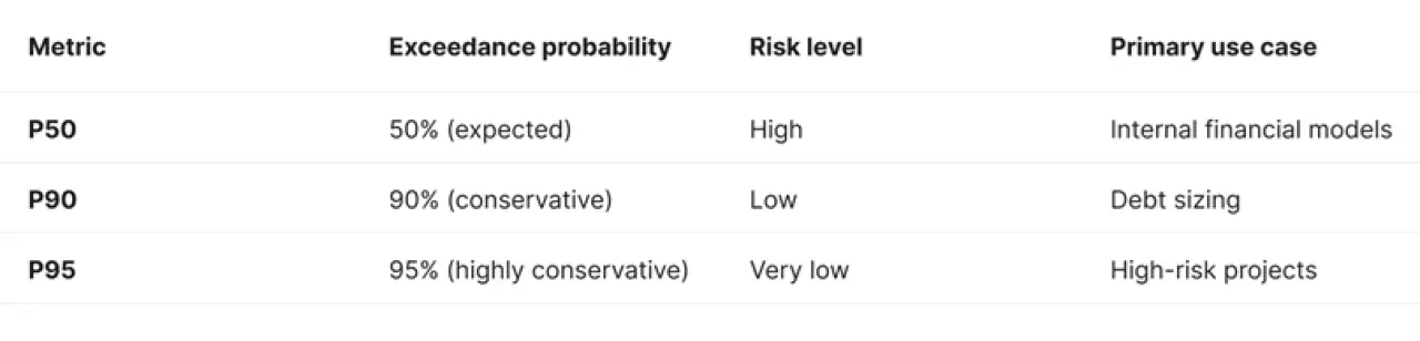
• P50: The expected annual production with a 50% probability that actual output will be higher or lower. Lenders often view P50 as too high-risk for debt sizing.

• P90 and P95: Conservative estimates representing the production level a plant is 90% or 95% certain to exceed.

Financial institutions typically size debt based on P90 to mitigate debt-service risk. While traditional assessments often carry a 5% to 11% uncertainty range, reducing this gap through high-fidelity modeling directly lowers interest rates on project debt and increases the total loan amount a project can secure.

P50 vs. P90 probability metrics

Minimizing Mean Bias Error (MBE) to increase debt capacity

The certainty of a P90 estimate is only as reliable as its underlying data. To justify a more aggressive (higher) P90 to investors, engineers must minimize the Mean Bias Error (MBE). 

This is achieved by cross-verifying at least two independent, high-resolution satellite meteorological datasets—such as SolarAnywhere or Meteonorm—against available on-site ground measurements. By reducing the "uncertainty delta" between the average P50 and the conservative P90, developers can unlock more capital while maintaining the same level of risk.

Finding the "sweet spot" for Net Present Value (NPV)

Once a reliable data foundation is established, accurate yield assessments allow engineers to optimize the system design specifically to maximize revenue. This involves identifying the "sweet spot" for yield by precisely calculating panel tilt and orientation to lower the Levelized Cost of Energy (LCOE). 

For example, studies have shown that reorienting panels just twice per year can increase annual production by 3% to 4.8%. These optimizations ensure that the project achieves the highest possible Return on Investment (ROI) for its stakeholders.

Establishing "ground truth" for warranty and insurance claims

Bankability also relies on the ability to recover capital during technical failures. Although only 0.05% of solar panels fail annually, high-fidelity yield assessments provide the necessary evidence to back up performance guarantee claims if output drops. 

Furthermore, if a system is damaged by environmental hazards like wind or hail, the initial assessment serves as the "ground truth" for insurers. It establishes exactly what the system would have produced before the damage, ensuring insurance payouts are sufficient to maintain project solvency.

Meteorological inputs: GHI, DNI, and bankable data

The foundation of any simulation is its irradiance data. Professional engineering differentiates between:

• Global Horizontal Irradiance (GHI): The primary driver for fixed-tilt systems.

• Direct Normal Irradiance (DNI): Critical for Single-Axis Trackers (SAT) and concentrating solar.

Selecting Bankable Data:

• The standard: Lenders require a Typical Meteorological Year (TMY) file derived from 10–20 years of satellite and ground records to account for inter-annual climate variability.

• Validation: Cross-verify satellite data (e.g., Solargis or SolarAnywhere) with on-site measurements to reduce MBE and uncertainty.

• Granularity: Sub-hourly data (5- to 15-minute resolution) is now the gold standard for accurately modeling inverter performance and midday clipping losses.

To better understand how these atmospheric variables impact your specific site coordinates, you can utilize a solar irradiance calculator to cross-verify satellite meteorological records with localized data.

The Digital Twin approach: 3D topographical modeling

Modern yield estimation has evolved from 2D approximations to Digital Twins—high-fidelity virtual replicas of the physical solar asset. Physics-based modeling calculates the electrical, optical, and thermal behavior of each individual module in real-time, accounting for:

• Topography-aware design: How the actual undulations of the site impact row-to-row shading.

• Dynamic variables: Localized wind speeds cooling the modules or spectral shifts throughout the day.

Calculating the expected energy output (E) involves a foundational formula that transitions from theoretical physics to grid-delivered AC power:

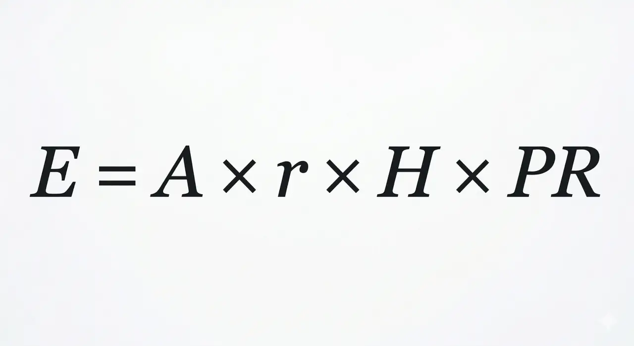
• A (Total solar panel area): The total physical surface area of the installed modules.

• r (Solar panel yield or efficiency): The percentage of sunlight that the specific panel can convert into electricity under standard test conditions.

• H (Annual average solar radiation): The amount of sunlight hitting the panels, often measured as Global Horizontal Irradiance (GHI) or Plane of Array (POA) irradiance.

• PR (Performance Ratio): A critical value—usually expressed as a percentage—that represents the total remaining energy after all system losses are deducted.

Deconstructing the "loss tree"

The Performance Ratio is the most important variable in the yield formula, as it represents the energy remaining after every systemic inefficiency is deducted. Achieving precision in solar simulations and loss calculations requires a granular understanding of how optical, spectral, and electrical factors interact to define the final AC output of a utility-scale plant.

1. Optical and spectral losses

These occur before photons are converted into electrons.

• Incidence Angle Modifier (IAM): Accounts for increased glass reflectivity when the sun is at an oblique angle.

• Soiling: Environmental accumulation (dust, pollen, bird droppings). NREL data suggests dust alone can trigger up to 7% annual energy loss in high-exposure regions.

• Shading: A high-impact "silent killer." Even 5% shading coverage can result in a 20-25% reduction in string-level output due to current mismatch.

2. Electrical and conversion efficiency

These losses occur during the Direct Current (DC) to Alternating Current (AC) transformation.

• Inverter clipping: Occurs when the DC/AC Ratio (Inverter Loading Ratio) exceeds the inverter's rated capacity during peak irradiance.

• DC/AC conversion: Energy lost as thermal dissipation during the inversion process.

• Resistive cabling losses: Professional modeling moves beyond fixed 1.5% estimates to calculate "dynamic" losses. This accounts for the specific conductor cross-sections (mm²) and the actual length of string runs to the inverter to preserve project margins.

For high-fidelity modeling in utility-scale solar projects, engineers utilize specialized methodologies that prioritize physical accuracy and detailed site-specific conditions to ensure project bankability.

The standard methodologies include:

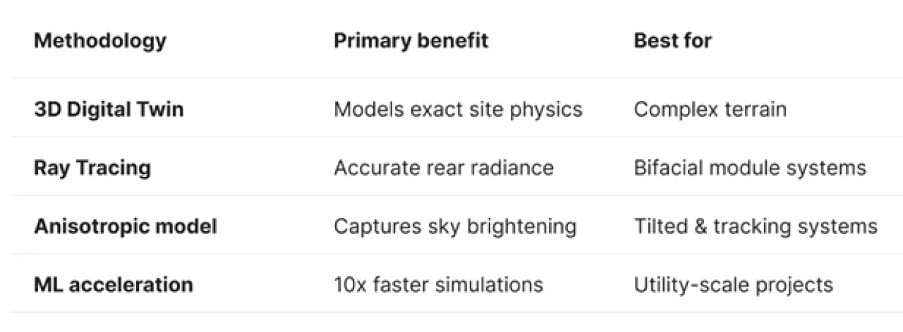
• Digital Twin modeling: Creates a high-fidelity virtual replica of the physical solar plant by importing the exact 3D layout, frame configurations, and terrain data from CAD environments to simulate real-world performance.

• Physics-based Ray Tracing: Explicitly calculates the paths of millions of light rays, accounting for both direct and reflected irradiance, which is essential for determining precise shading and rear-side albedo in bifacial systems.

• Anisotropic Transposition (Perez Model): A mathematical approach considered the "Gold Standard" for bankability that accounts for circumsolar and horizon brightening when calculating sunlight hitting a tilted panel.

• Integrated electrical-optical-thermal engines: Models real-time PV performance by simultaneously factoring in spectral shifts, temperature impacts on module efficiency, and electrical loss modeling.

• Terrain-following analysis: Adjusts modeling to follow the natural undulations of the land, allowing for more accurate shading and grading estimations on complex or irregular terrain.

• Machine Learning (ML) acceleration: Uses ML algorithms to remove redundant calculations in high-fidelity simulations, increasing processing speed by up to 10x without sacrificing the accuracy of the physics-based results.

With bankable energy yield assessments as their ultimate goal, engineers and analysts are progressively adopting integrated engines that factor in spectral shifts, temperature impacts, and complex electrical losses.

High-fidelity methodology comparison

To optimize solar project yield for maximal asset Return on Investment (ROI), engineers must focus on high-fidelity modeling and a "fail fast" development strategy to mitigate technical and financial risks.

Meteorological data & resource assessment

✅ Bankable source selection: Use high-resolution satellite data (e.g., Solargis, SolarAnywhere) with a minimum of 10–20 years of historical records.

✅ On-Site validation: Cross-reference satellite data with at least 12 months of high-quality on-site ground measurements to reduce Mean Bias Error (MBE).

✅ TMY file verification: Ensure the Typical Meteorological Year (TMY) reflects recent climate trends, including extreme weather events and aerosol variations.

✅ Granularity: Use sub-hourly (5 or 15-minute) data to accurately model inverter clipping and dynamic temperature effects.

Terrain & Digital Twin modeling

✅ High-fidelity topography: Utilize LiDAR-based topographical data with a resolution of 1 meter or better.

✅ Digital Twin construction: Ensure the yield model is a 3D virtual replica that accounts for every module's specific coordinates and elevation.

✅ Slope-aware layout: Verify that the layout follows natural contours to minimize expensive earthworks while accounting for slope-induced shading.

✅ 3D Ray Tracing: Use physics-based ray tracing rather than 2D approximations, essential for calculating back-side irradiance in bifacial systems.

Granular "loss tree" quantification

✅ Optical losses: Explicitly model Incidence Angle Modifier (IAM) losses, soiling based on regional rainfall/dust, and localized shading from trees or nearby structures.

✅ Spectral & LID: Account for light-induced degradation (LID) and spectral shifts specific to the chosen module chemistry.

✅ Dynamic DC losses: Calculate DC resistance based on the specific electrical stringing plan and real-world cable lengths, not a flat percentage.

✅ Inverter performance: Model efficiency curves and clipping losses accurately based on the project's DC/AC Ratio (typically 1.2–1.5).

Uncertainty & probability exceedance

✅ P90/P95 calculation: Provide conservative exceedance estimates for debt sizing; ensure the gap between P50 and P90 is mathematically justified by total project uncertainty.

✅ Inter-annual variability: Factor in the statistical standard deviation of the solar resource over the past two decades.

✅ Operational availability: Assume realistic downtime for O&M, grid outages, and component failures based on manufacturer data.

Advanced technology integration

✅ Tracker performance: If using single-axis trackers, verify the Terrain-Following capability to reduce shading and civil costs simultaneously.

✅ Bifacial gain: Validate "Albedo" assumptions using regional ground-cover data; avoid overestimating rear-side yield without site-specific soil analysis.

✅ BESS coupling: If the plant includes storage, simulate charge/discharge cycles to identify energy lost during the round-trip process.

By implementing these steps developers can secure project bankability while improving overall workflow efficiency. PVcase Yield makes these feats possible, ultimately helping to de-risk entire portfolios.